An intuitive guide to optimal transport, part II: the Wasserstein GAN made easy

No guide to optimal transport for machine learning would be complete without an explanation of the Wasserstein GAN (wGAN). In the first post of this series I explained the optimal transport problem in its primal and dual form. I concluded the post by proving the Kantorovich-Rubinstein duality, which provides the theoretical foundation of the wGAN. In this post I will provide an intuitive explanation of the concepts behind the wGAN and discuss their motivations and implications. Moreover, instead of using weight clipping like in the original wGAN paper, I will use a new form of regularization that is in my opinion closer to the original Wasserstein loss. Implementing the method using a deep learning framework should be relatively easy after reading the post. A simple Chainer implementation is available here. Let’s get started!

Why to use a Wasserstein divergence

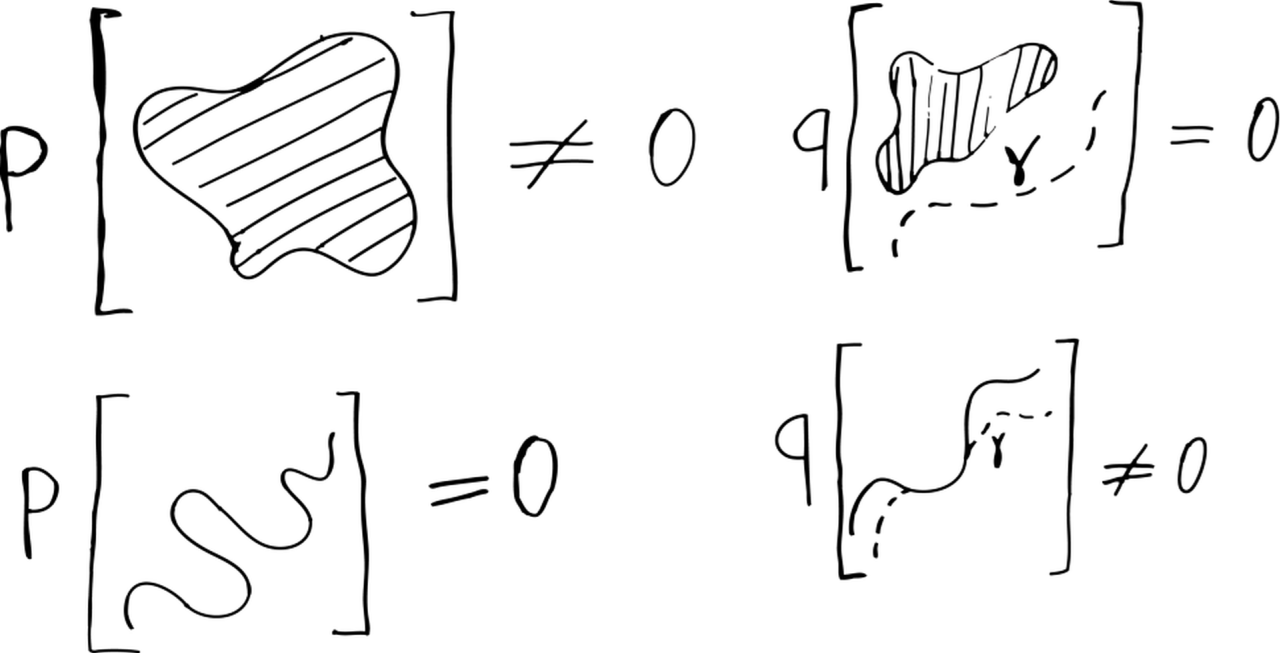
The original wGAN paper opens with a lengthy explanation of the advantages of the Wasserstein metric over other commonly used statistical divergences. While the discussion was rather technical, the take home message is simple: the Wasserstein metric can be used for comparing probability distributions that are radically different. What do I mean by different? The most common example is when two distributions have different support, meaning that they assign zero probability to different families of sets. For example, assume that $P(x)$ is a usual probability distribution on a two dimensional space defined by a probability density. All sets of zero volume (such as individual points and curves) in this space have zero probability under $p$. Conversely, $Q(x)$ is a weirder distribution that concentrates all its probability mass on a curve $\alpha$. All sets that do not contain the curve have zero probability under Q while some sets with zero volume have non-zero probability as far as they “walk along” the curve. I visualized this behavior in the following picture:

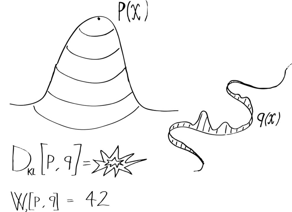
Now, these two distributions are very different from each other and they are pretty difficult to compare. For example, in order to compute their KL divergence we would need to calculate the density ratio $p(x)/q(x)$ for all points, but $Q$ does not even have a density with respect to the ambient space! However, we can still transport one distribution into the other using the optimal transport formalism that I introduced in the previous post! The Wasserstein distance between the two distributions is given by:

$$\mathcal{W}_2\[p,q]^2 = \inf_\gamma \int_{x_2 \in \alpha} \left( \int \left\lVert x_2 - x_1 \right\rVert^2_2 \gamma(x_2\vert x_1)dx_2 \right) dQ(x_1)~.$$

Let’s analyze this expression in detail. The inside integral is the average cost of transporting a point $x_1$ of the curve to a point $x_2$ of the ambient space under the transport map $\gamma(x_2\vert x_1)$. The outer integral is the average of this expected cost under the distribution $Q$ defined on the curve. We can summarize this in four step: 1) pick a point $x_1$ from the curve $\alpha$, 2) transport a particle from $x_1$ to $x_2$ with probability $\gamma(x_2\vert x_1)$, 3) compute the cost of transporting a particle from $x_1$ to $x_2$ and 4) repeat this many times and average the cost. Of course, in order to assure that you are transporting $Q$ to the target distribution $P$ you need to check that the marginalization constraint is satisfied:

$$\int_{x_2 \in \alpha} \gamma(x_2\vert x_1) dQ(x_1) = p(x)~,$$

meaning that sampling particles from $Q$ and then transporting them using $\gamma$ is equivalent to sampling particles directly from $P$. Note that the procedure does not care whether the distributions $P$ and $Q$ have the same support. Thus we can use the Wasserstein distance for comparing these extremely different distributions.

But is this relevant in real applications? Yes it definitely is. Actually most of the optimizations we perform in probabilistic machine learning involve distributions with different support. For example, the space of natural images is often assumed to live in a lower dimensional (hyper-)surface embedded in the pixel space. If this hypothesis is true, the distribution of natural images is analogous to our weird distribution $Q$. Training a generative model requires the minimization of some sort of divergence between the model and the real distribution of the data. The use of the KL divergence is very sub-optimal in this context since it is only defined for distributions that can be expressed in terms of a density. This could be one of the reasons why variational autoencoders perform worse than GANs on natural images.

The dual formulation of the Wasserstein distance

That was a long diversion, however I think it is important to properly understand the motivations behind the wGAN. Let’s now focus on the method! As I explained in the last post, the starting point for the wGAN is the dual formulation of the optimal transport problem. The dual formulation of the (1-)Wasserstein distance is given by the following formula:

$$\mathcal{W}_1\[p,q] = \text{sup}_{f \in L_c} \left\[ \int f(x) p(x) dx - \int f(x) q(x) dx \right] ~,$$

where $L$ is the set of Lipschitz continuous functions:

$$L = \left { f:\Re \rightarrow \Re \middle\vert \vert f(x_2) - f(x_1)\vert \leq \vert x_2 - x_1\vert \right}~.$$

The dual formulation of the Wasserstein distance has a very intuitive interpretation. The function $f$ has the role of a nonlinear feature map that maximally enhances the differences between the samples coming from the two distributions. For example, if $p$ and $q$ are distributions of images of male and female faces respectively, then $f$ will assign positive values to images with masculine features and these values will get increasingly higher as the input gets closer to a caricatural hyper-male face. In other words, the optimal feature map $f$ will assign a continuous score on a masculinity/femininity spectrum. The role of the Lipschitz constraint is to block $f$ from arbitrarily enhancing small differences. The constraint assures that if two input images are similar the output of $f$ will be similar as well. In the previous example, a minor difference in the hairstyle should not make an enormous difference on our masculine/feminine spectrum. Without this constraint the result would be zero when $p$ is equal to $q$ and $\infty$ otherwise since the effect of any minor difference can be arbitrarily enhanced by an appropriate feature map.

The Wasserstein GAN

The basic idea behind the wGAN is to minimize the Wasserstein distance between the sampling distribution of the data $p(x)$ and the distribution of images synthesized using a deep generator. Specifically, images are obtained by passing a latent variable $z$ through a deep generative model $g$ parameterized by the weights $\phi$. The resulting loss has the following form:

$$\mathcal{L}\[\phi] = \sup_{f \in L_c} \left[ \text{E}_{x \sim p(x)} \left\[ f(x) \right] - \text{E}_{z \sim p(z)} \left\[ f(g(z,\phi)) \right]\right] ~,$$

where $q(z)$ is a distribution over the latent space. As we saw in the last section, the dual formulation already contains the idea of a discriminator in the form of a nonlinear feature map $f$. Unfortunately it is not possible to obtain the optimal $f$ analytically. However, we can parameterize $f$ using a deep network and learn its parameters $\theta$ with stochastic gradient descent. This naturally leads to a min-max problem:

$$\inf_\phi \left[ \sup_\theta\left[ \text{E}_{x \sim p(x)} \left\[ f(x) \right] - \text{E}_{z \sim p(z)} \left\[ f(g(z,\phi)) \right] \right] \right]~.$$

In theory, the discriminator should be fully optimized every time we make an optimization step in the generator. However in practice we update $\phi$ and $\theta$ simultaneously. Isn’t this beautiful? The adversarial training naturally emerges from the abstract idea of minimizing the Wasserstein distance together with some obvious approximations. The last thing to do is to enforce the Lipschitz constraint in our learning algorithm. In the original GAN paper this is done by clipping the weights if they get bigger than a predefined constant. In my opinion, a more principled way is to relax the constraint and add an additional stochastic regularization term to the loss function:

$$\tilde{\mathcal{L}}\[\phi, \theta] = \mathcal{L}\[\phi, \theta] + \lambda \text{ReLu}\left(\vert f(x_2) - f(x_1)\vert - \vert x_2 - x_1\vert \right)^2~.$$

This term is zero when the constraint is fulfilled while it adds a positive value when it is not. The original strict constraint is formally obtained by tending $\lambda$ to infinity. In practice, we can optimize this loss using a finite value of $\lambda$.

Is the Wasserstein GAN really minimizing an optimal transport divergence?

The Wasserstein GAN is clearly a very effective algorithm that naturally follows from a neat theoretical principle. But does it really work by minimizing the Wasserstein distance between the generator and the data distribution? The dual formulation of the Wasserstein distance crucially relies on the fact that we are using the optimal nonlinear feature map $f$ under all possible Lipschitz continuous functions. The constraint makes an enormous difference. For example, if we use the same difference of expectation loss but we replace Lipschitz functions with continuous functions with values bounded between $-1$ and $1$ we obtain the total variation divergence. While training the wGAN we are actually restricting $f$ to be some kind of deep neural network with a fixed architecture. This constraint is enormously more restrictive that the sole Lipschitz constraint and it leads to a radically different divergence. The set of Lipschitz functions from images to real numbers is incredible flexible and does not induce any relevant inductive bias. The theoretically optimal $f$ can detect differences that are invisible to the human eye and does not assign special importance to differences that are very obvious for humans. Conversely, deep convolution networks have a very peculiar inductive bias that somehow matches the bias of the human visual system. Therefore, it is possible that the success of the wGAN is not really due to the mathematical properties of the Wasserstein distance but rather to the biases induced by the parameterization of the feature map (discriminator).

The anatomy of a good paper

The original Wasserstein GAN paper is a clear example of a beautiful machine learning publication, something that all machine learning researchers should be striving to be able to write. The starting point of the paper is a simple and elegant mathematical idea motivated by observations about the distribution of real data. The algorithm follows very naturally from the theory, with the adversarial scheme popping out from the formulation of the loss. Finally, the experimental section is very well made and the results are state-of-the-art. Importantly, there is nothing difficult in the paper and most of us could have pulled it off with just some initial intuition followed by hard work. I feel that there are still many low hanging fruits in our field and the key for grasping them is to follow the example of papers like this.