Music Genre Classification

Model AI Assignment
EAAI-12: Third Symposium on Educational Advances in Artificial Intelligence
Toronto, Ontario, Canada
July 23-24, 2012

Douglas Turnbull
Department of Computer Science
Ithaca College
dturnbull@ithaca.edu

Summary	Music Genre Classification: students explore the engaging topic of content-based music genre classification while developing practical machine learning skills
Topics	Main Focus: supervised learning, bag-of-feature-vector representation, the Gaussian classifier, k-Nearest Neighbor classifier, cross-validation, confusion matrix
Audience	Undergraduate students in an introductory course on artificial intelligence, machine learning, or information retrieval
Difficulty	Students must be familiar with file input/output, basic probability and statistics (e.g., multi-variate Gaussian distribution), and have a basic understanding of western popular music (e.g., rock vs. techno genres).
Strengths	Music is interesting. Most college-aged students have an iPod, use Pandora, go to live shows, share music with their friends, etc. To this end content-based music analysis is a fun, engaging, and relevant topic for just about every student. Using music, this assignment motivates a number of important machine learning topics that are useful for computer vision, recommender systems, multimedia information retrieval, and data mining.
Weaknesses	Requires a bit of file management to get started. However, sample Matlab code has been provided to help with file I/O.
Dependencies	This lab can be done using any programming languages though Matlab or Python (with the Numpy library) is recommended.
Variants	Data Mining Competition: can serve as a "bake-off" assignment where students can propose and implement their own classification approach. Undergraduate Research Project: music analysis is a hot research topic and students are often interested in learning more about it. Related projects might include using digital signal processing to directly analyze audio content, text-mining music blogs, collecting music information extracted from popular social networks (last.fm, Facebook), and building music recommendation applications (iTunes Genius, Pandora).

Index

• Overview
• Objectives
• Background Reading
• Details
• Discussion Questions
• Possible Extensions
• Final Remarks

In this lab, you will learn how a computer can automatically classify songs by genre through the analysis of the audio content. We provide a data set consisting of 150 songs where each song can be associated with one of the six genres.

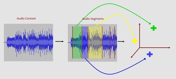
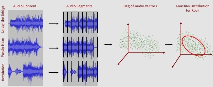
Each song is represented by a bag-of-feature-vectors. Each 12-dimensional feature vector represents the timbre, or "color", of the sound for a short (less than one second) segment of audio data. If we think about each feature vector as being a point in a 12-dimensional timbre space, then we can think of a song being a cloud of points in this same timbre space. Furthermore, we can think of many songs from a particular genre as occupying a region in this space. We will use a multivariate Gaussian probability distribution to model the occupying region of timbre for each genre.

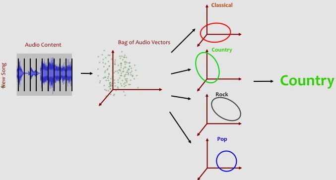
When we are given a new unclassified song, we calculate the probability of the song's bag-of-audio-feature-vectors under each of the six Gaussian genre models. We then predict that the genre with the highest probability. We can evaluate the accuracy of our Gaussian classifier by comparing how often the predicted genre matches the true genre for songs that were not originally used to create the Gaussian genre models.

1. important supervised learning concepts (training, evaluation, cross-validation)
2. the bag-of-feature-vector representation
3. a Gaussian classifier
4. a k-Nearest Neighbor classifier

For this lab in particular, below is a list of three good references related to content-based music genre classification:

1. Echo Nest Analyze Documentation - provides a background on how the timbre-based audio features are computed using digital signal processing. It also provides information about other available audio features related to rhythm, key, tempo, harmony and loudness.
2. Music Genre Classification of Audio Signals by Tzanetakis & Cook (2002)- a seminal work on the music genre classification problem. This paper is accessible to undergraduate AI students and provides them experience reading scholarly works.
3. Exploring Automatic Music Annotation with Acoustically-Objective Tags by Tingle, Kim, & Turnbull (2010) - a more recent music classification paper that connects the Tzanetakis paper with the Echo Nest audio features. This paper also serves as an example of how an undergraduate student researcher (Tingle) can make a contribution to the field of music information retrieval.

The main venue for music classification research is the International Society for Music Information Retrieval. If you are interested in reading more, the cummulative proceedings for 12+ years of research is online and publicly available for download.

In addition, the Music Information Retrieval Evaluation eXchange (MIREX) is an annual evaluation for various music information retrieval tasks. Each year, music classification is one of the most popular tasks and you can read about the best performing systems. If you develop a solid classification system, consider submitting it to MIREX next year!

Step 1: Load up the data

In the data/ directory, you will find six subdirectories for six genres of music: classical, country, jazz, pop, rock, and techno. Each folder contains 25 data files for 25 songs that are associated with the specific genre. The relationship between a song and a genre is determined by social tagging and obtained using the Last.fm API.

The files are formatted as follows:

# Perhaps Love - John Denver
0.0,171.13,9.469,-28.48,57.491,-50.067,14.833,5.359,-27.228,0.973,-10.64,-7.228
26.049,-27.426,-56.109,-95.41,-40.974,99.266,-5.217,-18.986,-27.03,59.921,60.989,-4.059
35.338,5.255,-40.244,-14.309,32.12,30.625,9.415,-8.023,-27.699,-45.148,23.829,20.7
...

where the first line starts with a # symbol followed by the song name and artist. You can hear samples of most songs using Spotify, the Apple iTunes Store, last.fm, YouTube or any other music hosting site. Each following line consists of 12 decimal numbers that together represent the audio content for a short, stable segment of music. You can think of these numbers as a 12-dimensional representation of the various frequencies that make up a musical note or chord in the song. There are between about 300 to about 1300 segments per song. This number depends on both the length of the song (i.e., longer songs tend to have more segments), but also on the beat (i.e., fast vs. slow tempo) and timbre (e.g., noisy vs. minimalist) of the music. Below is a visual representation of how we can represent a song as a bag-of-feature-vectors:

Your first step will be to load all 150 files into you program. The key will be to design a data structure that allows you to have access to each individual song's audio feature matrix (e.g, the time series of 12-dimensional audio feature vectors) as well as the metadata associated with each song (song name, artist name, genre).

Before Moving On: your program should load the audio feature matrices and associated metadata from the 150 data files.

Step 2: Learning a Gaussian Distribution for each Genre

For each genre, you will need to calculate a 12-dimensional mean vector and a 12x12-dimensional covariance matrix. These 12+144 numbers fully describe our probabilistic model for the genre. (Note: If some genre were more common than other genres, we would have to store this additional information in the model as well. This is sometimes called the prior probability of a genre.) Below is a visual representation of how we can model the audio content from a set of songs using a Gaussian distribution:

To start, we want to concatenate the audio features matrices for each of the 20 training songs. This is done by taking all of the rows from each of the feature matrices for the trainings songs associated with a genre and combining them into one large feature matrix. This will result in a large nx12-dimensional matrix where n will be between of 10,000 to 30,000 audio feature vectors (i.e., 20 songs times about 800 feature vectors per song.) You can then either use built-in math library functions to calculate the mean and covariance for this big data matrix or you can write the code from scratch. We will also want to use a built-in math function to calculate the inverse of the covariance matrix.

Note: Most programming languages (Matlab, Python-Numpy) have math libraries that provide useful mean, covariance, matrix transpose and matrix inverse functions. See the programming language documentation for details. To code these function from scratch, refer to an AI textbook, a statistics textbook, or Wikipedia for standard definitions of each concept.

Before Moving On: you should have one mean vector (12-dimensional), one covariance matrix (12x12-dimensional), and one inverse covariance matrix (12x12-dimensional) for each of the 6 genres.

Step 3: Predicting the Genre of a Song

For each audio feature vector, the unnormalized negative log likelihood (UNLL) is:

UNLL = (x - mean_genre) * inverse(cov_genre) * transpose(x - mean_genre)

where x is the 1x12 audio feature vector, mean_genre is the 1x12 mean vector calculate in step 2, and inverse(cov_genre) is the 12x12 inverse of the covariance matrix also calculated in step 2. Finally, we then find the average UNLL for all of the audio vectors of the song.

Once we have calculated the average-UNLL for a song under each of the 6 Gaussian genre models, we simply predict the genre associated with the smallest average-UNLL value. If the true genre matches the predicted genre, we have accurately classified the song.

Before Moving On: You should calculate the average-UNLL for each of the 30 test set songs and each of the 6 genre models.

Step 4: Evaluating Our Gaussian Classifiers

We can further explore the data by noting which genres are relatively easy to classify and which pairs of genres are often confused with one another. Try filling out the 6x6 confusion matrix to help you visualize this information better. One axis of this matrix represents the true genre label while the other axis represents the predicted label. The diagonal cells represent accurate predictions while the off-diagonal cells indicated which pairs of genres are likely to be confused with one another.

To probe deeper into the results, you can look at individual mistakes made by our classification system. For example, you may find that the system predicted a pop song as being a techno song. However, upon closer inspection, the specific pop song may have a strong synthesized beat that is characteristic of most techno songs. This kind of qualitative analysis can provide us with a better understanding of how music genres are related to one another.

Before Moving On: You should calculate the classification accuracy and confusion matrix for the Gaussian classifier.

(Optional) Step 5: Comparing Against a k-Nearest Neighbor Classifier

There are many algorithms that we can use to classify music by genre. One common and easy-to-implement classifier is call the k-Nearest Neighbor (kNN) classifier. You can implement this classifier and see how its performance compares to the Gaussian classifier. Here is how it works:

First, instead of learning a Gaussian Distribution for each genre, estimate the parameters (mean vector, covariance matrix) for each song in the training set. This will produce 120 Gaussian distributions.

Second, calculate the average-UNLL between each of the 30 test set songs and each of the 120 training set Gaussian distribution. This will result in a 30x120 dimensional matrix.

Third, pick a small odd number k (e.g., k = 1, 3, or 5). Then, for each test set song, find the "k nearest neighbor" songs in the training set. These are the k songs in the training set with the smallest average-UNLL.

Fourth, use the genre labels for these nearest neighbor to predict the label of the test set song. For example, if the the five nearest neigbor of a test set song are associated with the genres [pop, rock, rock, jazz, rock], we would predict the song is a rock song because three of the nearest neighbors are rock. We can break ties randomly or use some other heuristic (e.g., closest neighbor wins).

Once you have predicted a genre for each of the test set songs using the kNN classifier, you can evaluate the classifier using accuracy as described in step 5.

1. What assumptions about the data do we make when we model the date using a Gaussian distribition?
2. When do you expect that a Gaussian will work well and when do you think it will not work well?
3. What values of k work best for the kNN classifier?
4. Based on your results from this assignment, which classifier (Gaussian or kNN) works best for the task of Music Genre Classification?
5. Why do you think each classifier performed as well (or as poorly ) as it did?
6. Can you think of ways that you can modify the classifiers so that you might improve performance?

1. Explore Your Own Music: Using the Echo Nest API, you can upload your own music. Also, if you want to check out a huge data set of music, you should check out the Million Song Dataset.
2. Try Additional Audio Features: You can also use the Echo Nest API to get additional audio features that relate to tempo, key, mode, harmony, etc. Note that the file names in the data/ directory are Echo Nest Track IDs so you can obtain these features without owning a copy of the individual audio tracks. Alternatively, you use digital signal processing to calculate your own audio features.
3. Use Social Information: While this lab focused on content-based music classification, you can collect social information (blog entries, rating data, social tags) from a number of public APIs (Echo Nest, Last.fm, Facebook, etc.)
4. Develop Alternative Classifiers: In this lab, we focused on a Gaussian classifier and a k-nearest neighbor classifier. However, this is just one of many classification systems. Other common classifiers include a support vector machine (SVM), a Gaussian mixture model(GMM), or a hidden Markov model (HMM). Better yet, invent your own classification algorithm.

If you have any questions or suggestions, feel free to email Doug Turnbull at dturnbull@ithaca.edu .