Last edited February 26, 2017.

I really, really like the Wasserstein GAN paper. I know it’s already gotten a lot of hype, but I feel like it could use more.

I also think the theory in the paper scared off a lot of people, which is a bit of a shame. This is my contribution to make the paper more accessible, while hopefully retaining the thrust of the argument.

Why Is This Paper Important?

There’s a giant firehose of machine learning papers - how do you decide which ones are worth reading closely?

For Wasserstein GAN, it was mostly compelling word of mouth.

• The paper proposes a new GAN training algorithm that works well on the common GAN datasets.
• Said training algorithm is backed up by theory. In deep learning, not all theory-justified papers have good empirical results, but theory-justified papers with good empirical results have really good empirical results. For those papers, it’s very important to understand their theory, because the theory usually explains why they perform so much better.
• I heard that in Wasserstein GAN, you can (and should) train the discriminator to convergence. If true, it would remove needing to balance generator updates with discriminator updates, which feels like one of the big sources of black magic for making GANs train.
• The paper shows a correlation between discriminator loss and perceptual quality. This is actually huge if it holds up well. In my limited GAN experience, one of the big problems is that the loss doesn’t really mean anything, thanks to adversarial training, which makes it hard to judge if models are training or not. Reinforcement learning has a similar problem with its loss functions, but there we at least get mean episode reward. Even a rough quantitative measure of training progress could be good enough to use automated hyperparam optimization tricks, like Bayesian optimization. (See this post and this post for nice introductions to automatic hyperparam tuning.)

Additionally, I buy the argument that GANs have close connections to actor-critic reinforcement learning. (See Pfau & Vinyals 2017.) RL is definitely one of my research interests. Also, GANs are taking over the world; I should probably keep an eye on GAN papers anyways.

At this point, you may want to download the paper yourself, especially if you want more of the theoretical details. To aid anyone who takes me up on this, the section names in this post will match the ones in the paper.

Introduction

The paper begins with background on generative models.

When learning generative models, we assume the data we have comes from some unknown distribution $P_r$$P_r$. (The r stands for real.) We want to learn a distribution $P_\theta$$P_\theta$ that approximates $P_r$$P_r$, where $\theta$$\theta$ are the parameters of the distribution.

You can imagine two approaches for doing this.

• Directly learn the probability density function $P_\theta$$P_\theta$. Meaning, $P_\theta$$P_\theta$ is some differentiable function such that $P_\theta(x) \ge 0$$P_\theta(x) \ge 0$ and $\int_x P_\theta(x)\, dx = 1$$\int_x P_\theta(x)\, dx = 1$. We optimize $P_\theta$$P_\theta$ through maximum likelihood estimation.
• Learn a function that transforms an existing distribution $Z$$Z$ into $P_\theta$$P_\theta$. Here, $g_\theta$$g_\theta$ is some differentiable function, $Z$$Z$ is a common distribution (usually uniform or Gaussian), and $P_\theta = g_\theta(Z)$$P_\theta = g_\theta(Z)$.

The paper starts by explaining why the first approach runs into problems.

Given function $P_\theta$$P_\theta$, the MLE objective is

In the limit, this is equivalent to minimizing the KL-divergence $KL(P_r \| P_\theta)$$KL(P_r \| P_\theta)$.

Aside: Why Is This True?

Recall that for continuous distributions $P$$P$ and $Q$$Q$, the KL divergence is

In the limit (as $m \to \infty$$m \to \infty$), samples will appear based on the data distribution $P_r$$P_r$, so

(Derivations in order: limit of summation turns into integral, flip max to min by negating, add a constant that doesn’t depends on $\theta$$\theta$, and apply definition of KL divergence.)

Note that if $Q(x) = 0$$Q(x) = 0$ at an $x$$x$ where $P(x) > 0$$P(x) > 0$, the KL divergence goes to $+\infty$$+\infty$. This is bad for the MLE if $P_\theta$$P_\theta$ has low dimensional support, because it’ll be very unlikely that all of $P_r$$P_r$ lies within that support. If even a single data point lies outside $P_\theta$$P_\theta$’s support, the KL divergence will explode.

To deal with this, we can add random noise to $P_\theta$$P_\theta$ when training the MLE. This ensures the distribution is defined everywhere. But now we introduce some error, and empirically people have needed to add a lot of random noise to make models train. That kind of sucks. Additionally, even if we learn a good density $P_\theta$$P_\theta$, it may be computationally expensive to sample from $P_\theta$$P_\theta$.

This motivates the latter approach, of learning a $g_\theta$$g_\theta$ (a generator) to transform a known distribution $Z$$Z$. The other motivation is that it’s very easy to generate samples. Given a trained $g_\theta$$g_\theta$, simply sample random noise $z \sim Z$$z \sim Z$, and evaluate $g_\theta(z)$$g_\theta(z)$. (The downside of this approach is that we don’t explicitly know what $P_\theta$$P_\theta$, but in practice this isn’t that important.)

To train $g_\theta$$g_\theta$ (and by extension $P_\theta$$P_\theta$), we need a measure of distance between distributions.

(Note: I will use metric, distance function, and divergence interchangeably. I know this isn’t technically accurate. In particular metric and divergence mean different things. I apologize in advance, the three are all heavily conflated in my head.)

Different metrics (different definitions of distance) induce different sets of convergent sequences. We say distance $d$$d$ is weaker than distance $d'$$d'$ if every sequence that converges under $d'$$d'$ converges under $d$$d$.

Looping back to generative models, given a distance $d$$d$, we can treat $d(P_r, P_\theta)$$d(P_r, P_\theta)$ as a loss function. Minimizing $d(P_r, P_\theta)$$d(P_r, P_\theta)$ with respect to $\theta$$\theta$ will bring $P_\theta$$P_\theta$ close to $P_r$$P_r$. This is principled as long as the mapping $\theta \mapsto P_\theta$$\theta \mapsto P_\theta$ is continuous (which will be true if $g_\theta$$g_\theta$ is a neural net).

Different Distances

We know we want to minimize $d$$d$, but how do we define $d$$d$? This section compares various distances and their properties.

Now, I’ll be honest, my measure theory is pretty awful. And the paper immediately starts talking about compact metric sets, Borel subsets, and so forth. This is admirable from a theory standpoint. However, in machine learning, we’re usually working with functions that are “nice enough” (differentiable almost everywhere), and can therefore ignore many of the precise definitions without destroying the argument too much. As long as we aren’t doing any bullshit like the Cantor set, we’re good.

On to the distances at play.

• The Total Variation (TV) distance is

• The Kullback-Leibler (KL) divergence is

  $KL(P_r\|P_g) = \int_x \log\left(\frac{P_r(x)}{P_g(x)}\right) P_r(x) \,dx$ $$KL(P_r\|P_g) = \int_x \log\left(\frac{P_r(x)}{P_g(x)}\right) P_r(x) \,dx$$

  This isn’t symmetric. The reverse KL divergence is defined as $KL(P_g \| P_r)$$KL(P_g \| P_r)$.

• The Jenson-Shannon (JS) divergence: Let $M$$M$ be the mixture distribution $M = P_r/2 + P_g/2$$M = P_r/2 + P_g/2$. Then

  $JS(P_r,P_g) = \frac{1}{2}KL(P_r\|P_m)+\frac{1}{2}KL(P_g\|P_m)$ $$JS(P_r,P_g) = \frac{1}{2}KL(P_r\|P_m)+\frac{1}{2}KL(P_g\|P_m)$$

• Finally, the Earth Mover (EM) or Wasserstein distance: Let $\Pi(P_r, P_g)$$\Pi(P_r, P_g)$ be the set of all joint distributions $\gamma$$\gamma$ whose marginal distributions are $P_r$$P_r$ and $P_g$$P_g$. Then.

  $W(P_r, P_g) = \inf_{\gamma \in \Pi(P_r ,P_g)} \mathbb{E}_{(x, y) \sim \gamma}\big[\:\|x - y\|\:\big]$ $$W(P_r, P_g) = \inf_{\gamma \in \Pi(P_r ,P_g)} \mathbb{E}_{(x, y) \sim \gamma}\big[\:\|x - y\|\:\big]$$

Aside: What’s Up With The Earth Mover Definition?

The EM distance definition is a bit opaque. It took me a while to understand it, but I was very pleased once I did.

First, the intuitive goal of the EM distance. Probability distributions are defined by how much mass they put on each point. Imagine we started with distribution $P_r$$P_r$, and wanted to move mass around to change the distribution into $P_g$$P_g$. Moving mass $m$$m$ by distance $d$$d$ costs $m\cdot d$$m\cdot d$ effort. The earth mover distance is the minimal effort we need to spend.

Why does the infimum over $\Pi(P_r, P_g)$$\Pi(P_r, P_g)$ give the minimal effort? You can think of each $\gamma \in \Pi$$\gamma \in \Pi$ as a transport plan. To execute the plan, for all $x,y$$x,y$ move $\gamma(x,y)$$\gamma(x,y)$ mass from $x$$x$ to $y$$y$.

Every strategy for moving weight can be represented this way. But what properties does the plan need to satisfy to transform $P_r$$P_r$ into $P_g$$P_g$?

• The amount of mass that leaves $x$$x$ is $\int_y \gamma(x,y) \,dy$$\int_y \gamma(x,y) \,dy$. This must equal $P_r(x)$$P_r(x)$, the amount of mass originally at $x$$x$.
• The amount of mass that enters $y$$y$ is $\int_x \gamma(x,y) \,dx$$\int_x \gamma(x,y) \,dx$. This must equal $P_g(y)$$P_g(y)$, the amount of mass that ends up at $y$$y$.

This shows why the marginals of $\gamma \in \Pi$$\gamma \in \Pi$ must be $P_r$$P_r$ and $P_g$$P_g$. For scoring, the effort spent is $\int_x \int_y \gamma(x,y) \| x - y \| \,dy\,dx = \mathbb{E}_{(x,y) \sim \gamma}\big[\|x - y\|\big]$$\int_x \int_y \gamma(x,y) \| x - y \| \,dy\,dx = \mathbb{E}_{(x,y) \sim \gamma}\big[\|x - y\|\big]$ Computing the infinum of this over all valid $\gamma$$\gamma$ gives the earth mover distance.

Now, the paper introduces a simple example to argue why we should care about the Earth-Mover distance.

Consider probability distributions defined over $\mathbb{R}^2$$\mathbb{R}^2$. Let the true data distribution be $(0, y)$$(0, y)$, with $y$$y$ sampled uniformly from $U[0,1]$$U[0,1]$. Consider the family of distributions $P_\theta$$P_\theta$, where $P_\theta = (\theta, y)$$P_\theta = (\theta, y)$, with $y$$y$ also sampled from $U[0, 1]$$U[0, 1]$.

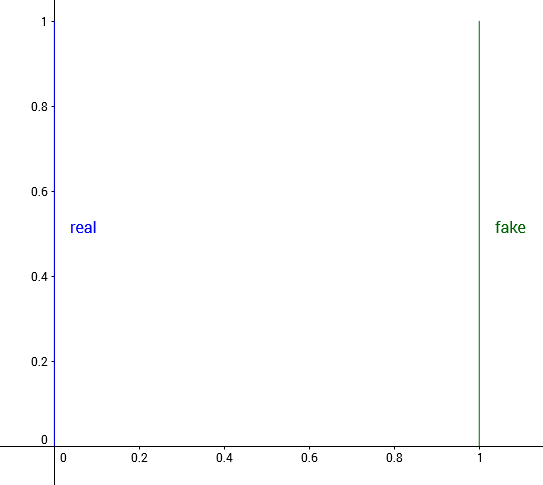
Real and fake distribution when $\theta = 1$$\theta = 1$

We’d like our optimization algorithm to learn to move $\theta$$\theta$ to $0$$0$, As $\theta \to 0$$\theta \to 0$, the distance $d(P_0, P_\theta)$$d(P_0, P_\theta)$ should decrease. But for many common distance functions, this doesn’t happen.

• Total variation: For any $\theta \neq 0$$\theta \neq 0$, let $A = \{(0, y) : y \in [0,1]\}$$A = \{(0, y) : y \in [0,1]\}$. This gives

• KL divergence and reverse KL divergence: Recall that the KL divergence $KL(P\|Q)$$KL(P\|Q)$ is $+\infty$$+\infty$ if there is any point $(x,y)$$(x,y)$ where $P(x,y) > 0$$P(x,y) > 0$ and $Q(x,y) = 0$$Q(x,y) = 0$. For $KL(P_0 \| P_\theta)$$KL(P_0 \| P_\theta)$, this is true at $(\theta, 0.5)$$(\theta, 0.5)$. For $KL(P_\theta \| P_0)$$KL(P_\theta \| P_0)$, this is true at $(0, 0.5)$$(0, 0.5)$.

• Jenson-Shannon divergence: Consider the mixture $M = P_0/2 + P_\theta/2$$M = P_0/2 + P_\theta/2$, and now look at just one of the KL terms.

For any $x,y$$x,y$ where $P_0(x,y) \neq 0$$P_0(x,y) \neq 0$, $M(x,y) = \frac{1}{2}P_0(x,y)$$M(x,y) = \frac{1}{2}P_0(x,y)$, so this integral works out to $\log 2$$\log 2$. The same is true of $KL(P_\theta \| M)$$KL(P_\theta \| M)$, so the JS divergence is

• Earth Mover distance: Because the two distributions are just translations of one another, the best way transport plan moves mass in a straight line from $(0, y)$$(0, y)$ to $(\theta, y)$$(\theta, y)$. This gives $W(P_0, P_\theta) = |\theta|$$W(P_0, P_\theta) = |\theta|$

This example shows that there exist sequences of distributions that don’t converge under the JS, KL, reverse KL, or TV divergence, but which do converge under the EM distance.

This example also shows that for the JS, KL, reverse KL, and TV divergence, there are cases where the gradient is always $0$$0$. This is especially damning from an optimization perspective - any approach that works by taking the gradient $\nabla_\theta d(P_0, P_\theta)$$\nabla_\theta d(P_0, P_\theta)$ will fail in these cases.

Admittedly, this is a contrived example because the supports are disjoint, but the paper points out that when the supports are low dimensional manifolds in high dimensional space, it’s very easy for the intersection to be measure zero, which is enough to give similarly bad results.

This argument is then strengthened by the following theorem.

Let $P_r$$P_r$ be a fixed distribution. Let $Z$$Z$ be a random variable. Let $g_\theta$$g_\theta$ be a deterministic function parametrized by $\theta$$\theta$, and let $P_\theta = g_\theta(Z)$$P_\theta = g_\theta(Z)$. Then,

1. If $g$$g$ is continuous in $\theta$$\theta$, so is $W(P_r, P_\theta)$$W(P_r, P_\theta)$.
2. If $g$$g$ is sufficiently nice, then $W(P_r, P_\theta)$$W(P_r, P_\theta)$ is continuous everywhere, and differentiable almost everywhere.
3. Statements 1-2 are false for the Jensen-Shannon divergence $JS(P_r, P_\theta)$$JS(P_r, P_\theta)$ and all the KLs.

You’ll need to refer to the paper to see what “sufficiently nice” means, but for our purposes it’s enough to know that it’s satisfied for feedfoward networks that use standard nonlinearites. Thus, out of JS, KL, and Wassertstein distance, only the Wasserstein distance has guarantees of continuity and differentiability, which are both things you really want in a loss function.

The second theorem shows that not only does the Wasserstein distance give better guarantees, it’s also the weakest of the group.

Let $P$$P$ be a distribution, and $(P_n)_{n \in \mathbb{N}}$$(P_n)_{n \in \mathbb{N}}$ be a sequence of distributions. Then, the following are true about the limit.

1. The following statements are equivalent.
   • $\delta(P_n, P) \to 0$$\delta(P_n, P) \to 0$ with $\delta$$\delta$ the total variation distance.
   • $JS(P_n,P) \to 0$$JS(P_n,P) \to 0$ with $JS$$JS$ the Jensen-Shannon divergence.
2. The following statements are equivalent.
   • $W(P_n, P) \to 0$$W(P_n, P) \to 0$.
   • $P_n \rightarrow P$$P_n \rightarrow P$, where $\rightarrow$$\rightarrow$ represents convergence in distribution for random variables.
3. $KL(P_n \| P) \to 0$$KL(P_n \| P) \to 0$ or $KL(P \| P_n) \to 0$$KL(P \| P_n) \to 0$ imply the statements in (1).
4. The statements in (1) imply the statements in (2).

Together, this proves that every distribution that converges under the KL, reverse-KL, TV, and JS divergences also converges under the Wasserstein divergence. It also proves that a small earth mover distance corresponds to a small difference in distributions.

Combined, this shows the Wasserstein distance is a compelling loss function for generative models.

Wasserstein GAN

Unfortunately, computing the Wasserstein distance exactly is intractable. Let’s repeat the definition.

The paper now shows how we can compute an approximation of this.

A result from Kantorovich-Rubinstein duality shows $W$$W$ is equivalent to

where the supremum is taken over all $1$$1$-Lipschitz functions.

Aside: What Does Lipschitz Mean?

Let $d_X$$d_X$ and $d_Y$$d_Y$ be distance functions on spaces $X$$X$ and $Y$$Y$. A function $f: X \to Y$$f: X \to Y$ is $K$$K$-Lipschitz if for all $x_1, x_2 \in X$$x_1, x_2 \in X$,

Intuitively, the slope of a $K$$K$-Lipschitz function never exceeds $K$$K$, for a more general definition of slope.

If we replace the supremum over $1$$1$-Lipschitz functions with the supremum over $K$$K$-Lipschitz functions, then the supremum is $K \cdot W(P_r, P_\theta)$$K \cdot W(P_r, P_\theta)$ instead. (This is true because every $K$$K$-Lipschitz function is a $1$$1$-Lipschitz function if you divide it by $K$$K$, and the Wasserstein objective is linear.)

The supremum over $K$$K$-Lipschitz functions $\{f : \|f\|_L \le K\}$$\{f : \|f\|_L \le K\}$ is still intractable, but now it’s easier to approximate. Suppose we have a parametrized function family $\{f_w\}_{w \in \mathcal{W}}$$\{f_w\}_{w \in \mathcal{W}}$, where $w$$w$ are the weights and $\mathcal{W}$$\mathcal{W}$ is the set of all possible weights. Further suppose these functions are all $K$$K$-Lipschitz for some $K$$K$. Then we have

For optimization purposes, we don’t even need to know what $K$$K$ is! It’s enough to know that it exists, and that it’s fixed throughout training process. Sure, gradients of $W$$W$ will be scaled by an unknown $K$$K$, but they’ll also be scaled by the learning rate $\alpha$$\alpha$, so $K$$K$ will get absorbed into the hyperparam tuning.

If $\{f_w\}_{w \in \mathcal{W}}$$\{f_w\}_{w \in \mathcal{W}}$ contains the true supremum among $K$$K$-Lipschitz functions, this gives the distance exactly. This probably won’t be true. In that case, the approximation’s quality depends on what $K$$K$-Lipschitz functions are missing from $\{f_w\}_{w \in \mathcal{W}}$$\{f_w\}_{w \in \mathcal{W}}$.

Now, let’s loop all this back to generative models. We’d like to train $P_\theta = g_\theta(Z)$$P_\theta = g_\theta(Z)$ to match $P_r$$P_r$. Intuitively, given a fixed $g_\theta$$g_\theta$, we can compute the optimal $f_w$$f_w$ for the Wasserstein distance. We can then backprop through $W(P_r, g_\theta(Z))$$W(P_r, g_\theta(Z))$ to get the gradient for $\theta$$\theta$.

The training process has now broken into three steps.

• For a fixed $\theta$$\theta$, compute an approximation of $W(P_r, P_\theta)$$W(P_r, P_\theta)$ by training $f_w$$f_w$ to convergence.
• Once we find the optimal $f_w$$f_w$, compute the $\theta$$\theta$ gradient $-\mathbb{E}_{z \sim Z}[\nabla_\theta f_w(g_\theta(z))]$$-\mathbb{E}_{z \sim Z}[\nabla_\theta f_w(g_\theta(z))]$ by sampling several $z \sim Z$$z \sim Z$.
• Update $\theta$$\theta$, and repeat the process.

There’s one final detail. This entire derivation only works when the function family $\{f_w\}_{w\in\mathcal{W}}$$\{f_w\}_{w\in\mathcal{W}}$ is $K$$K$-Lipschitz. To guarantee this is true, we use weight clamping. The weights $w$$w$ are constrained to lie within $[-c, c]$$[-c, c]$, by clipping $w$$w$ after every update to $w$$w$.

The full algorithm is below.

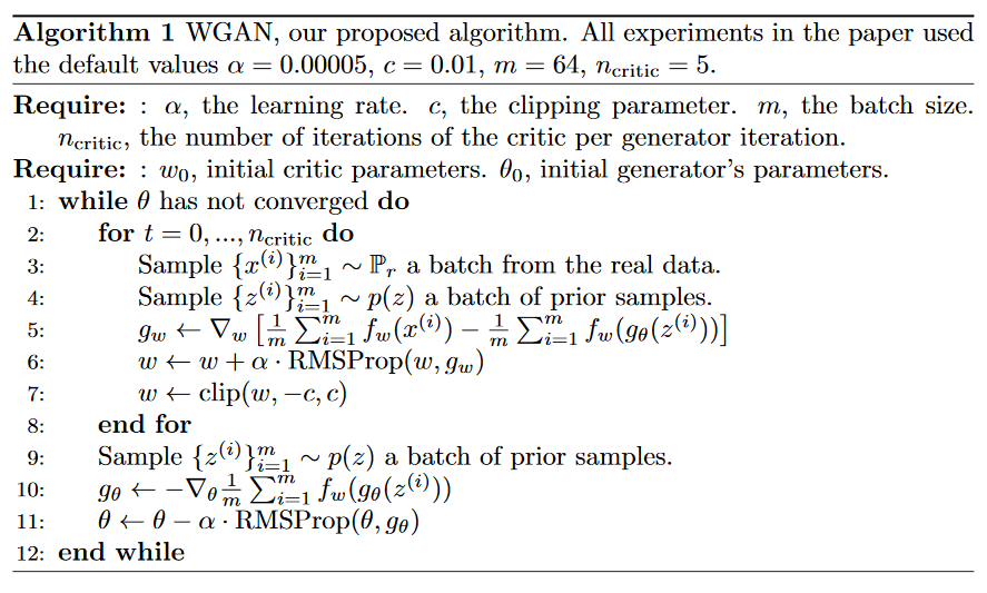
Aside: Compare & Contrast: Standard GANs

Let’s compare the WGAN algorithm with the standard GAN algorithm.

• In GANS, the discriminator maximizes

  $\frac{1}{m} \sum_{i=1}^m \log D(x^{(i)}) + \frac{1}{m} \sum_{i=1}^m \log (1 - D(g_\theta(z^{(i)})))$ $$\frac{1}{m} \sum_{i=1}^m \log D(x^{(i)}) + \frac{1}{m} \sum_{i=1}^m \log (1 - D(g_\theta(z^{(i)})))$$

  where we constraint $D(x)$$D(x)$ to always be a probabiity $p \in (0, 1)$$p \in (0, 1)$.

In WGANs, nothing requires $f_w$$f_w$ to output a probability. This explains why the authors tend to call $f_w$$f_w$ the critic instead of the discriminator - it’s not explicitly trying to classify inputs as real or fake.

• The original GAN paper showed that in the limit, the maximum of the discriminator objective above is the Jenson-Shannon divergence, up to scaling and constant factors.

In WGANs, it’s the Wasserstein distance instead.

• Although GANs are formulated as a min max problem, in practice we we never train $D$$D$ to convergence. In fact, usually the discriminator is too strong, and we need to alternate gradient updates between $D$$D$ and $G$$G$ to get reasonable generator updates.

We aren’t updating $G$$G$ against the Jenson-Shannon divergence, or even an approximation of the Jenson-Shannon divergence, we’re updating $G$$G$ against an objective that kind of aims towards the JS divergence, but doesn’t go all the way. It certainly works, but in light of the points this paper makes about gradients of the JS divergence, it’s a bit surprising it does work.

In contrast, because the Wasserstein distance is differentiable nearly everywhere, we can (and should) train $f_w$$f_w$ to convergence before each generator update, to get as accurate an estimate of $W(P_r, P_\theta)$$W(P_r, P_\theta)$ as possible. (The more accurate $W(P_r, P_\theta)$$W(P_r, P_\theta)$ is, the more accurate the gradient $\nabla_\theta W(P_r, P_\theta)$$\nabla_\theta W(P_r, P_\theta)$.)

Empirical Results

First, the authors set up a small experiment to showcase the difference between GAN and WGAN. There are two 1D Gaussian distributions, blue for real and green for fake. Train a GAN discriminator and WGAN critic to optimality, then plot their values over the space. The red curve is the GAN discriminator output, and the cyan curve is the WGAN critic output.

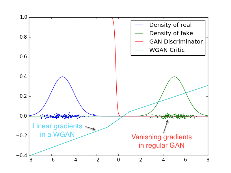
Both identify which distribution is real and which is fake, but the GAN discriminator does so in a way that makes gradients vanish over most of the space. In contrast, the weight clamping in WGAN gives a reasonably nice gradient over everything.

Next, the Wasserstein loss seems to correlate well with image quality. Here, the authors plot the loss curve over time, along with the generated samples.

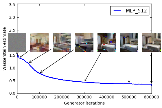
After reading through the paper, this isn’t too surprising. Since we’re training the critic $f_w$$f_w$ to convergence, these critic’s value should be good approximations of $K \cdot W(P_r, P_\theta)$$K \cdot W(P_r, P_\theta)$, where $K$$K$ is whatever the Lipschitz constant is. As argued before, a low $W(P_r, P_\theta)$$W(P_r, P_\theta)$ means $P_r$$P_r$ and $P_\theta$$P_\theta$ are “close” to one another. It would be more surprising if the critic value didn’t correspond to visual similarity.

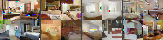
The image results also look quite good. Compared to the DCGAN baseline on the bedroom dataset, it performs about as well.

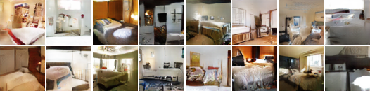
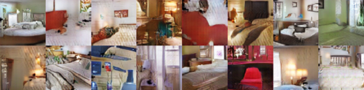
Top: WGAN with the same DCGAN architecture. Bottom: DCGAN

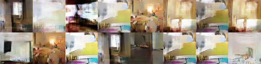
If we remove batch norm from the generator, WGAN still generates okay samples, but DCGAN fails completely.

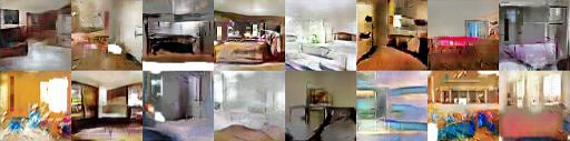
Top: WGAN with DCGAN architecture, no batch norm. Bottom: DCGAN, no batch norm.

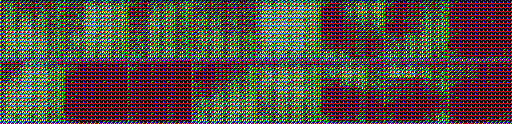
Finally, we make the generator a feedforward net instead of a convolutional one. This keeps the number of parameters the same, while removing the inductive bias from convolutional models. The WGAN samples are more detailed, and don’t mode collapse as much as standard GAN. In fact, they report never running into mode collapse at all for WGANs!

Top: WGAN with MLP architecture. Bottom: Standard GAN, same architecture.

Follow-Up Questions

The read-through of the paper ends here. If you’re interested in the Related Work, or the theorem proofs in the Appendix, you’ll need to read the paper.

This is a rich enough paper to have several natural follow-up questions.

The weights in $f_w$$f_w$ are clamped to $[-c, +c]$$[-c, +c]$. How important is $c$$c$ for performance? Based on lurking /r/MachineLearning, the tentative results say that low $c$$c$ trains more reliably, but high $c$$c$ trains faster when it does work. I imagine it’s because there’s a discrepancy between $\{f_w\}_{w\in\mathcal{W}}$$\{f_w\}_{w\in\mathcal{W}}$ and $\{f: \|f\|_L \le K\}$$\{f: \|f\|_L \le K\}$, and that discrepancy changes with $c$$c$. There could be interesting work in describing that discrepancy, or in finding ways to bring $\{f_w\}_{w\in\mathcal{W}}$$\{f_w\}_{w\in\mathcal{W}}$ closer to $K$$K$-Lipschitz functions while still be optimizable.

Given a fixed critic architecture and fixed $c$$c$ for clamping, can we quantitatively compare different generators by computing the Wasserstein estimate of both? Again, remember there’s an approximation error from optimizing over $\{f_w: w \in \mathcal{W}\}$$\{f_w: w \in \mathcal{W}\}$ instead of $\{f: \|f\|_L \le K\}$$\{f: \|f\|_L \le K\}$, so we may not be able to do much. However, because we fix both the critic architecture and $c$$c$, the hope is that most of the error is some universal error that appears in all distributions. If the approximation error doesn’t change too much between distributions, this would give a way to judge generation quality without relying on Mechanical Turk. (And if the error does change a lot, it would probably be interesting to investigate when that happens.)

The constant $K$$K$ depends on both $c$$c$ and the model architecture, and therefore we can’t directly compare the critics between models with different architectures. Is there a way to estimate $K$$K$? Recall the critic objective converges to $K \cdot W(P_r, P_\theta)$$K \cdot W(P_r, P_\theta)$, so dividing by $K$$K$ would normalize the difference between architectures.

(This actually seems pretty straightforward. Take either a random generator or pretrained generator, then train critics $f_w$$f_w$ from varying architectures and compare their final values. Again, the approximation error could complicate this, but this could be a way to analyze the approximation error itself. Given a few different generators, the change in estimated $K$$K$ between different distributions would show how important the distribution is to the approximation error.)

How important is it to train the critic to convergence? A converged critic gives the most accurate gradient, but it takes more time. In settings where that’s impractical, can a simple alternating gradient scheme work?

What ideas from this work are applicable to actor-critic RL? At a first glance, I’m now very interested in investigating the magnitude of the actor gradients. If they tend to be very large or very small, we may have a similar saturation problem, and adding a Lipschitz bound through weight clamping could help.

These ideas apply not just to generative models, but to general distribution matching problems. Are there any low-hanging distribution matching problems that use the Jenson-Shannon or KL divergence instead of the Wasserstein distance? One example of this is the Generative Adversarial Imitation Learning paper. After a decent amount of theory, it derives a GAN-like algorithm for imitation learning. Switching the discriminator to a WGAN approach may give some straightforward wins.