An Introduction to Monte Carlo Techniques in Artificial Intelligence - Part II

Todd W. Neller, Gettysburg College Department of Computer Science

Monte Carlo (MC) techniques have become important and pervasive in the work of AI practitioners.  In general, they provide a relatively easy means of providing deep understanding of complex systems as long as important events are not infrequent. 

Consider this non-exhaustive list of areas of work with relevant MC techniques:

• General: Monte Carlo simulation for probabilistic estimation
• Machine Learning: Monte Carlo reinforcement learning
• Uncertain Reasoning: Bayesian network reasoning with Gibbs Sampling, a Markov Chain Monte Carlo method
• Robotics: Monte Carlo localization
• Search: Monte Carlo tree search
• Game Theory: MC regret-based techniques

Herein, we will recommend readings and provide novel exercises to support the experiential learning of the third of these uses of MC techniques: Bayesian network reasoning with Gibbs Sampling, a Markov Chain Monte Carlo method.  Through these exercises, we hope that the student gains a deeper understanding of the strengths and weaknesses of these techniques, is able to add such techniques to their problem-solving repertoire, and can discern appropriate applications.

Prerequisite Knowledge

• Directed acyclic graphs (DAGs) (any Data Structures textbook)
• Axioms of probability (Russell and Norvig, Artificial Intelligence: A Modern Approach (AIMA), 3th ed., Pearson, Upper Saddle River, New Jersey, USA, 2010, section 13.2)
• Conditional probabilities and conditional probability tables (CPTs) (Russell and Norvig, section 14.1)

Supplementary Readings

• Bayesian networks: (pick one or more)
  • Russell and Norvig, AIMA 3e, section 14.1-14.2
  • Wikipedia article on Bayesian networks
  • Kevin Murphy's "A Brief Introduction to Graphical Models and Bayesian Networks" webpage, Representation section up to "Bayes nets with discrete and continuous nodes"
  • Other online sources are available as well.
• Gibbs sampling: (first reference recommended but others are possible supplements as noted):
  • Pearl, Judea. Research Note: "Evidential Reasoning Using Stochastic Simulation of Causal Models", AIJ Vol. 32 Issue 2, May 1987, pp. 245-257, Elsevier, Essex, UK.
    • or: Pearl, Judea. Probabilistic Reasoning in Intelligent Systems: Networks of Plausible Inference, Revised 2nd Printing, Morgan Kaufmann, San Francisco, California, USA, 1988, Table 1 (p. 197), section 4.4.3 (pp. 210-216, up to "Justifying the Computations")
  • Russell and Norvig, AIMA 3e, section 14.5.2 (pp. 535-536)
    • Note: GIBBS-ASK queries one nonevidence variable.  The project below queries all nonevidence variables, and additionally normalizes over summed conditional probabilities used for sampling to show more rapid convergence.
  • Koller and Friedman, Probabilistic Graphical Models: Principles and Techniques, MIT Press, Cambridge, Massachussetts, USA, 2010, sections 12.3.1-12.3.3 (pp. 505-515)
    • Note: Gibbs sampling is initially presented more generally for Markov chains. Specialization to the use of the Markov blanket is given in 12.3.3, but without revised pseudocode.  Further, the pseudocode returns the sample without normalization, and without conditional probability samples as with the previous reference.
  • Other online sources are available as well.

The Problem: Bayesian Network Reasoning

Let us suppose you are a doctor seeking to make a cancer diagnosis based on internal effects of the cancer and external symptoms of those effects.  The external symptoms are often easy and/or inexpensive to observe.  The internal effects of the cancer may be relatively more difficult and/or expensive to observe.  It would be useful to be able to reason from symptoms backwards to obtain probabilities on internal effects and the cancer diagnosis itself.  This is the type of example given in Judea Pearl's research note, "Evidential Reasoning Using Stochastic Simulation of Causal Models".

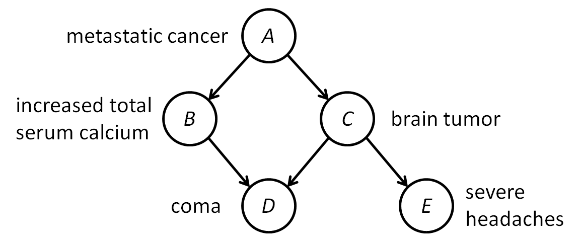
For Pearl's example, he establishes 5 discrete, true/false-valued variables concerning whether or not the patient has (A) metastatic cancer, (B) increased total serum calcium, (C) a brain tumor, (D) a coma, and (E) a severe headache.  One simple approach to this problem would be to collect a lot of data concerning these variables in different patients, remove those data that do not match the evidence at hand (e.g. the patient has a severe headache and is not in a coma), and see how frequently the other variables are true or false.  One general difficulty of this approach is that, for complex problems, we may have much evidence which would match few or no prior cases, and thus our data would be insufficient to reason with.

If, however, we can identify simple, direct causal relationships between our variables, and then compute or otherwise provide a good estimate the frequencies of variable assignments in these relationships, we are more able to perform sound probabilistic reasoning with limited data.  This is one of the motivations for representing relationships between discrete-valued variables (i.e. variables that take on a finite number of values) as Bayesian networks, which we shall now describe by example.

Let us suppose the following: Whether or not a patient has (B) increased total serum calcium is directly influenced only by whether or not the patient has (A) metastatic cancer. Whether or not a patient has (C) a brain tumor is also directly influenced only by whether or not the patient has (A) metastatic cancer.  Whether or not a patient is in a (D) coma is directly influenced by whether or not the patient has (B) increased total serum calcium and/or (C) a brain tumor.  Whether or not a patient has (E) a severe headache is directly influenced only by whether or not the patient has (C) a brain tumor.  For this simple, illustrative example, we can represent variables as nodes and direct influence as edges in a directed acyclic graph (DAG): 

When a node has a single parent (e.g. B has single parent A) in the DAG, this means that, lacking further evidence, the probability of B depends only on the value of A.  We may express this by conditional probability equations, e.g. "P(B=true|A=false) = .2" and "P(B=true|A=true) = .8", which mean "The probability that B is true given that A is false is .2", and "The probability that B is true given that A is true is .8", respectively.  Note that since all of our variables are boolean, we do not then need to provide conditional probability equations for  P(B=false|A=false) or P(B=false|A=true), because B must have a value and, given our conditional probabilities for B being true, we simply substract these values from 1 to derive these values (.8 and .2, respectively).   Put simply, the probability of a boolean variable being false in a given situation is one minus the probability of it being true in that same situation.

These same conditional probability equations concerning B may also be expressed in different notations, e.g. "P(B|!A)" or "P(+B|-A) = .2" or "P(+B|˜A) = .2" or "P(+B|¬A) = .2".  Pearl expressed his conditional probabilities using this latter style with lowercase variables:

P(a):	P(+a) = .20
P(b|a):	P(+b|+a) = .80	P(+b|¬a) = .20
P(c|a):	P(+c|+a) = .20	P(+c|¬a) = .05
P(d|c,b):	P(+d|+b,+c) = .80	P(+d|¬b,+c) = .80
	P(+d|+b,¬c) = .80	P(+d|¬b,¬c) = .05
P(e|c):	P(+e|+c) = .80	P(+e|¬c) = .60

From this information, we may compute joint probabilities, that is, the probability of any truth assignment to all variables.  For example, if we wish to know the probability of b and d being false while all other variables are true, then because of these influence relationships:

P(+a,¬b,+c,¬d,+e)
= P(+a) * P(¬b|+a) * P(+c|+a) * P(¬d|¬b,+c) * P(+e|+c)
= P(+a) * (1 - P(+b|+a)) * P(+c|+a) * (1 - P(+d|¬b,+c)) * P(+e|+c)
= .20 * (1 - .80) * .20 * (1 - .80) * .80
= .20 * .20 * .20 * .20 * .80
= .00128

Then we may, for small numbers of variables, compute all such joint probabilities that match our evidence (keeping evidence variables constant and iterating through all nonevidence variable possible combinations), and sum them in order to reason probabilistically.  However, as the number of nonevidence variables increases, the number of joint probabilities that would need to be computed grows exponentially, so this approach is only practical for problems with few nonevidence variables.

These relationships may also be expressed in the form of conditional probability tables that, for these discrete true/false values, resemble truth tables:

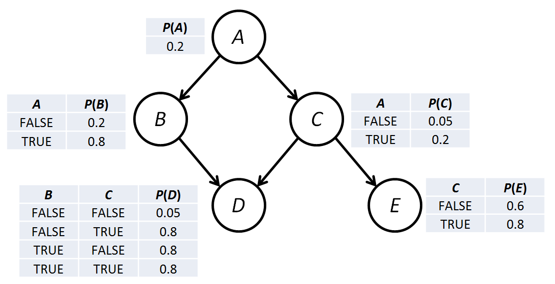
The directed acyclic graph (DAG) of direct influence relationships together with conditional probability tables (CPTs) for each node variable based on all possible parent node variable values is called a Bayesian network.  A method for constructing Bayesian networks is given in Russell & Norvig, AIMA, 3e, section 14.2.1, but we can summarize by recommending that one builds the network by beginning with an independent causal variable node, and then progressively adding nodes whose variables are also independently causal or are influenced solely by node variables already in the network.  Iterating from earliest causal variables through intermediate effect variables to latest effect variables will yield a network that is sparse and captures the local structure that makes the algorithm that follows efficient.

A brief word on generalization to multivalued discrete variables: While this project concerns only two-valued Boolean variables for simplicity, this does not preclude any of the following discussion and algorithmic work from relevance to three-or-more-valued discrete variables.  In such cases, the CPTs must include enough rows to capture all possible value combinations of parent(s) (e.g. brain tumor variable C could have values "none", "small", "medium", and "large") and the CPTs must include enough columns for all but one of the possible child variable values (e.g. severe headache variable E could instead be an integer-valued pain scale, including a column for all but one pain scale value, which can be computed by subtracting the sum of other value probabilities from one.).  In all that follows, we may generalize to three-or-more-valued discrete variables, but for simplicity we will assume Boolean variables throughout.

The Markov Blanket

One last observation is that a sparse Bayesian network with relatively few edges between nodes means that computation of the probability of a node can depend entirely on knowledge of nodes that are "local" to it in some sense.  To understand what we mean by locality, let us focus on node B of Pearl's Bayesian network.  In the CPTs above, note which CPTs contain any reference to B, and then note all nodes that occur in those tables.  We can see that the CPT for node B itself contains information from node A, which is B's only parent.  We can also see that the CPT for node D contains information from node B, one of D's parents, and additionally contains information from node C, D's other parent.

In general, the CPTs that refer to a node N will either (1) be for N itself and refer to N's parents, or (2) be for each of N's children and refer to all of N's childrens' parents, called N's mates.  Thus all CPT's relating to N will also relate to N's parents, N's children, and N's mates.  N's parents, children, and mates are collectively refered to as N's Markov blanket. 

The important property to understand about the Markov blanket to understand is that, given variable values for all variables in N's Markov blanket, you can compute the probability of N:

• Relative likelihood of N being true from Markov blanket: First, compute the parental probability of N being true by looking up the appropriate entry in N's CPT given the values of N's parents.  Then, for each child C, multiply this value by the entry of C's CPT for C's value given N's mates values and using true for N's value.  Keep this product as a measure of the relative likelihood that N is true given the values of N's Markov blanket nodes.
• Relative likelihood of N being false from Markov blanket: Next, do the same for N being false. Compute the parental probability of N being false by looking up the appropriate entry in N's CPT given the values of N's parents.  Then, for each child C, multiply this value by the entry of C's CPT for C's value given N's mates values and using false for N's value.  Keep this product as a measure of the relative likelihood that N is false given the values of N's Markov blanket nodes.
• Probability of N being true from Markov blanket: Finally, we can normalize these relative likelihoods and obtain the conditional probability that N is true given the values of N's Markov blanket nodes. Simply divide the relative likelihood that N is true by the sum of both relative likelihoods.  

Worked mathematical examples of this process are given within this excerpt of Pearl's book Probabilistic Reasoning in Intelligent Systems: Networks of Plausible Inference, section "Illustrating the Simulation Scheme" (pp. 213-216).

Looking at the CPTs that involve N, it becomes clear that, given values for all nodes in N's Markov blanket, the probability of N itself can be determined and does not involve values of nodes beyond it's Markov blanket.  Put another way, knowledge of N's Markov blanket variable values makes N conditionally independent of all other variable values.  The introduction (or disappearance) of evidence beyond the given full evidence of the Markov blanket is irrelevant to the computation of N's probability.  It is said that N's Markov blanket evidence "blocks" the influence of all other nodes.

A Solution: Gibbs Sampling

This local computation of the probability of a node value from values of its Markov blanket is the core operation of the Gibbs Sampling algorithm, an instance of the class of Markov Chain Monte Carlo (MCMC) algorithms.  To understand what is common in MCMC, we begin by describing a Markov chain.  A Markov chain is a random process that probabilistically transitions from state to state, but has a property that it is "memoryless" in that the transition probability from one state to the state depends only on the current state and not from prior history.

Consider a robotic vacuum on a square floor that is discretized into n-by-n grid cells, and let us simply model the robot's movement as randomly staying in place or moving one cell horizontally, vertically, or diagonally in the grid.  No matter where we start the robot, after sufficient time (called mixing time) we cannot tell where the robot started.  If we collect all positions the robot occupies on each time step after such mixing time, the distribution will estimate the true probability distribution over all robot states, and one will see that corner and side state probabilities are less than interior state probabilities for this process.

The Monte Carlo simulation of a Markov chain and the use of the distribution of states resulting to gain insights to the Markov's chain's distribution or to sample this distribution, is what is common to Markov Chain Monte Carlo algorithms.

In our case, we would like to, given Bayesian network evidence nodes that are set at a specific value, compute an estimate of the probability of all nonevidence nodes.  In the Gibbs sampling application of MCMC ideas, the state of the Bayesian network is not a single node in the network.  Rather, the state is an assignment to all nonevidence variables.  (Evidence variables are "clamped" at their evidence value.)  The question then remains: "How can we randomly walk among variable assignments so that the frequency of a variables values over time converges to the true probability of the variable given the evidence?" 

Remarkably, the solution is simple:

• Initially assign all nonevidence variables arbitrarily, and assign all evidence variables to evidence values. 
• For a large number of iterations:
  • For each nonevidence node N (ordering isn't important):
    • Compute the probability of N's values given the current values of nodes in its Markov blanket.
    • Assign a new value to N given the computed value probabilities.
    • Collect both the value probabilities and the assigned value for N.

At the end of the process:

• The proportion of iterations that N is assigned a given value approximates the true probability of that value for N.
• The average of the probabilities computed for each value assigned to N also approximates the true probabilities for each value assigned to N.  These average probabilities also converge more quickly.

This is a high-level overview of the Gibbs sampling algorithm.  If you have not already, you should read Judea Pearl's illustration of the process for his cancer Bayesian network from this excerpt of his book Probabilistic Reasoning in Intelligent Systems: Networks of Plausible Inference, section "Illustrating the Simulation Scheme" (pp. 213-216).  This provides a worked mathematical example to help you understand Gibbs sampling in detail.

In the exercises below, you will implement Gibbs sampling and perform experiments with it that will exercise your knowledge representation skills, and demonstrate different reasoning patterns and concepts.  We will not be concerned with mixing time, and will use statistics from all iterations of the algorithm.  Use at least 1000000 iterations per query.

Exercises

1. Stochastic Simulation with Gibbs Sampling:  Implement Gibbs sampling of a Bayesian network as described in Section 4.4.3 of "Probabilistic Reasoning in Intelligent Systems" by Judea Pearl.  Much convenient groundwork has been done for you.  In file modelai-mcmc-dist.zip, you will find (among other things) an Eclipse project containing a collection of Java files that parse input and construct a Bayesian network data structure for you.  You should only be concerned with implementing the simulate() method in BNGibbsSampler.java. Do not modify other parts of the code.
• Input Format: Input Format:  To specify Pearl's cancer Bayesian network with evidence of no coma and a severe headache, you would create a file like pearl.in:

P(a) = {.20}
P(b|a) = {.20, .80}
P(c|a) = {.05, .20}
P(d|b,c) = {.05, .80, .80, .80}
P(e|c) = {.60, .80}
evidence
-d
e

The BNF grammar for the input file is as follows:
<inputFile>  ←  <cptList> [ "evidence" <evidenceList>] <EOF>
<cptList>  ←  ( <cpt> )+
<cpt> ←  "P" "(" <varName> [ "|" <parentList> ] ")" "=" "{" <pvalueList> "}"
<parentList>  ←  <varName> ( "," <varName> )*
<pvalueList>  ←  <pvalue> ( "," <pvalue> )*
<evidenceList>  ←  ( <evidence> )*
<evidence>  ←  "-" <varName> | <varName>
where <varName> is an alphanumeric variable name starting with a letter, and <pvalue> is a probability value.

Since this implementation deals with Boolean values only, CPTs are organized like truth tables.  If one takes parents in the order listed in the CPT and replace them with 0 or 1 for false and true, respectively, and then concatenate them to a binary number, that number's value is the index for probability lookup in the array that follows.  For example, suppose we wish to know the probability of d being true given that b is true and c is false.  The CPT specification in the pearl.in file above is "P(d|b,c) = {.05, .80, .80, .80}".  Parents are listed in the order b,c, so replacing these with 1 for b (true) and 0 for c (false) and concatenating them yields binary number 10, or decimal number 2, which indicates that the relevant probability for d being true is at 0-based index 2 (the third entry in the list of probabilities).  So the probability of d being true would be .8.  The probability of d being false given the same values for b and c would be (1-.8) = .2.

CPT entries should be topologically sorted so that variables are not used as conditioning variables before their own CPT entry has been defined.  For example, if "P(b|a)  = ..." came before "P(a) = ..." above, the parser would complain.  Evidence is optional, but if there is no evidence, you may omit the keyword "evidence" as well.  Variable names are case sensitive.

Output Format:  Output format should mimic that of the sample output files.  For example, the output from the command
java BNGibbsSampler 10000000 2000000 < pearl.in > pearl.out
would yield output of the form below (but with different estimated probability values):


BNNode a:
  value: false
  parents: (none)
  children: b c
  CPT: 0.2
BNNode b:
  value: false
  parents: a
  children: d
  CPT: 0.2 0.8
BNNode c:
  value: false
  parents: a
  children: d e
  CPT: 0.05 0.2
BNNode d:
  EVIDENCE
  value: false
  parents: b c
  children: (none)
  CPT: 0.05 0.8 0.8 0.8
BNNode e:
  EVIDENCE
  value: true
  parents: c
  children: (none)
  CPT: 0.6 0.8
______________________________________________________________________
After iteration 200000:
Variable, Average Conditional Probability, Fraction True
a, 0.0971144285711284, 0.096385
b, 0.09707124999969938, 0.09655
c, 0.031003729284424134, 0.031815
______________________________________________________________________
After iteration 400000:
Variable, Average Conditional Probability, Fraction True
a, 0.09726980357149692, 0.096775
b, 0.09716282142863672, 0.0970625
c, 0.03109983597229418, 0.0315075
______________________________________________________________________
After iteration 600000:
Variable, Average Conditional Probability, Fraction True
a, 0.09744563095330394, 0.09715
b, 0.09732005952473075, 0.097475
c, 0.031158255337808277, 0.03146
______________________________________________________________________
After iteration 800000:
Variable, Average Conditional Probability, Fraction True
a, 0.09743473214411201, 0.09719375
b, 0.09732475000125447, 0.0974875
c, 0.031153070745652163, 0.03141625
______________________________________________________________________
After iteration 1000000:
Variable, Average Conditional Probability, Fraction True
a, 0.09725659285855631, 0.096923
b, 0.09716166428712687, 0.097158
c, 0.031087865742980978, 0.031275

The first command line parameter is the number of iterations.  The second is the iteration frequency for reporting results.  If only the first command line parameter is given, the frequency is set to the same, i.e. only one final report will be given.  Default values for the first and second parameters are 1000000 and 200000.

Initial Bayesian network node information is printed for you.  In your reporting (by frequency or after last iteration) for each non-evidence node, print both the average conditional probability and the fraction of iterations the variable has been assigned true.

As your first exercise, implement the Gibb Sampling algorithm such that your output for pearl.in is similar to that above.  For guidance, the exact conditional probability of variable a for the above problem is .0972762646.  Remember that you should only be concerned with implementing the simulate() method in BNGibbsSampler.java. Do not modify other parts of the code.  Also, study the BNNode javadoc documentation. You will find that you begin simulate() with a Bayesian network data structure of BNNodes pre-built from the standard input grammar specification, and that your algorithm will take far less than 100 lines of code to implement if you use the BNNode class well. 

Here is a detailed outline for your algorithm:

• Build a list of nonevidence nodes (from BNNode.nodes) and randomly assign them values.
• Initialize statistics for each nonevidence node.
• For the given number of iterations:
  • For each nonevidence node:
    • Set the node to true and get its CPT table entry using the BNNode cptLookup method.
    • For each child of the node, multiply the value by the child's CPT table entry (or one minus the table entry for false children)
    • Store this value as the relative likelihood of the node being true.
    • Repeat the process with the node set to false in order to compute the relative likelihood of the node being false.
    • Normalize in order to compute the probability of the node being true.  Add this for a statistical average for this node.
    • Select a new random value for this node according to this probability.  Tally this assignment if true for future node statistics.
  • If it's a reporting iteration or the last iteration, print the current statistics for each nonevidence node as shown above.



2. Representation and reasoning: Use your BNGibbsSampler.java implementation for this and the following questions.  Encode the Bayesian network of Russell & Norvig Figure 14.2 for input to the program above as file alarm.in.  What are the probabilities of nonevidence variables with no evidence?  With Mary calling?  With Mary calling and positive evidence of an earthquake?
    
3. Conditional independence: Describe what evidence and/or lack thereof is necessary for nodes b and c to be conditionally independent in the given Bayesian network (pearl.in).  Put another way, for nodes a, d, and e, which combinations of these in evidence cause evidence of b to have no effect on c (and vice versa)? Experiment to test your answer.
    
4. Diagnostic inference concerns querying a nonevidence variable that is an ancestor of an evidence variable, reasoning backward from effects to causes.  How does the introduction of true evidence of d affect the probability of a compared to our pearl.in network with no evidence?
   
   
5. Causal inference concerns querying a nonevidence variable that is a descendant of an evidence variable, reasoning forward from causes to effects.  How does the introduction of false evidence of a affect the probability of d compared to our pearl.in network with no evidence?
   
   
6. Intercausal inference (also called "explaining away") concerns a querying common cause variables of the same evidence effect variable.  Suppose we have evidence only of a coma (d) in our pearl.in network.  What are the probabilities of b and c?  Suppose then that we learn that the patient has a brain tumor (c).  What is the new probability of them having increased total serum calcium (b)?  Suppose instead that we learn that the patient has increased total serum calcium (b)? What is the new probability of them having a brain tumor (c)?
   
   
7. Mixed inference concerns a queried nonevidence variable that is both a descendant and an ancestor of evidence variables.  For example, if the patient has no metastatic cancer (a) but is in a coma (d), what is the probability of the patient having a brain tumor (c) in our pearl.in network?
   
   
8. A weakness of Gibbs sampling: As with many Monte Carlo simulation algorithms, one must be careful when improbable (but not impossible) events are of great importance.  In the Bayes network tree (tree.in) defined below, what are the true probabilities of each variable (assuming no evidence)?  Perform Gibbs sampling with different orders of magnitudes of iterations (e.g.  10000, 100000, 1000000, 10000000), share your results, and reflect on what they teach.

   P(a) = {.1}
   P(b|a) = {0, .1}
   P(c|a) = {0, .1}
   P(d|b) = {0, .1}
   P(e|b) = {0, .1}
   P(f|d) = {0, .1}
   P(g|d) = {0, .1}
   P(h|f) = {0, .1}
   P(i|f) = {0, .1}
   P(j|h) = {0, .1}
   P(k|h) = {0, .1}

9. D-separation (advanced): Read section 2.4 ("D-separation") of  Ross Shachter's "Bayes-Ball: ..." article and demonstrate three different ways evidence or lack thereof can D-separate two nodes, causing them to become conditional independent of each other.  Using the alarm.in Bayesian network of Russell & Norvig Figure 14.2, show how: 
   • evidence of an alarm creates or eliminates conditional independence between a burglary and John calling
   • evidence of an alarm creates or eliminates conditional independence between John calling and Mary calling
   • evidence of an alarm and/or call(s) creates or eliminates conditional independence between a burglary and an earthquake

Further Explorations in Markov Chain Monte Carlo Algorithms

There are many examples of Markov Chain Monte Carlo (MCMC) algorithms that you can explore further:

• Simulated Annealing is an MCMC algorithm used for global optimization and especially combinatorial optimization.  Learn about Simulated Annealing in an application to logic maze design.
• WalkSAT is a MCMC algorithm for seeking a satisfying truth assignment for the SAT problem.  A project that encourages implementation of WalkSAT concerns  reasoning about the deductive boardgame Clue.
• The PageRank algorithm, which was responsible for Google's rise, invites another application of MCMC through simulated web surfing.  There are a variety of PageRank assignments available online, but here is the basic idea:
  • Represent a set of webpages as nodes in a directed graph where a edge is between node i and node j if the webpage of node i has a link to the webpage of node j.
  • Pick a random node as your initial webpage.
  • For many iterations:
    • Surf the directed graph from your current node to an adjacent node, choosing among adjacent nodes with equal probability.  If a page has no links travel to any node with equal probability.  Count your visits to each node.
  • Compute the fraction of time a node is visited as an estimate of the relative imporantance of that page in the set of pages.

As one can see, applications of Markov Chain Monte Carlo are many and varied.  When a probability distribution seems difficult to sample or compute, consider designing a random process that has your desired distribution as a steady state over time, and start iterating!